Surfing: The Physics of Being Carried by a Wave

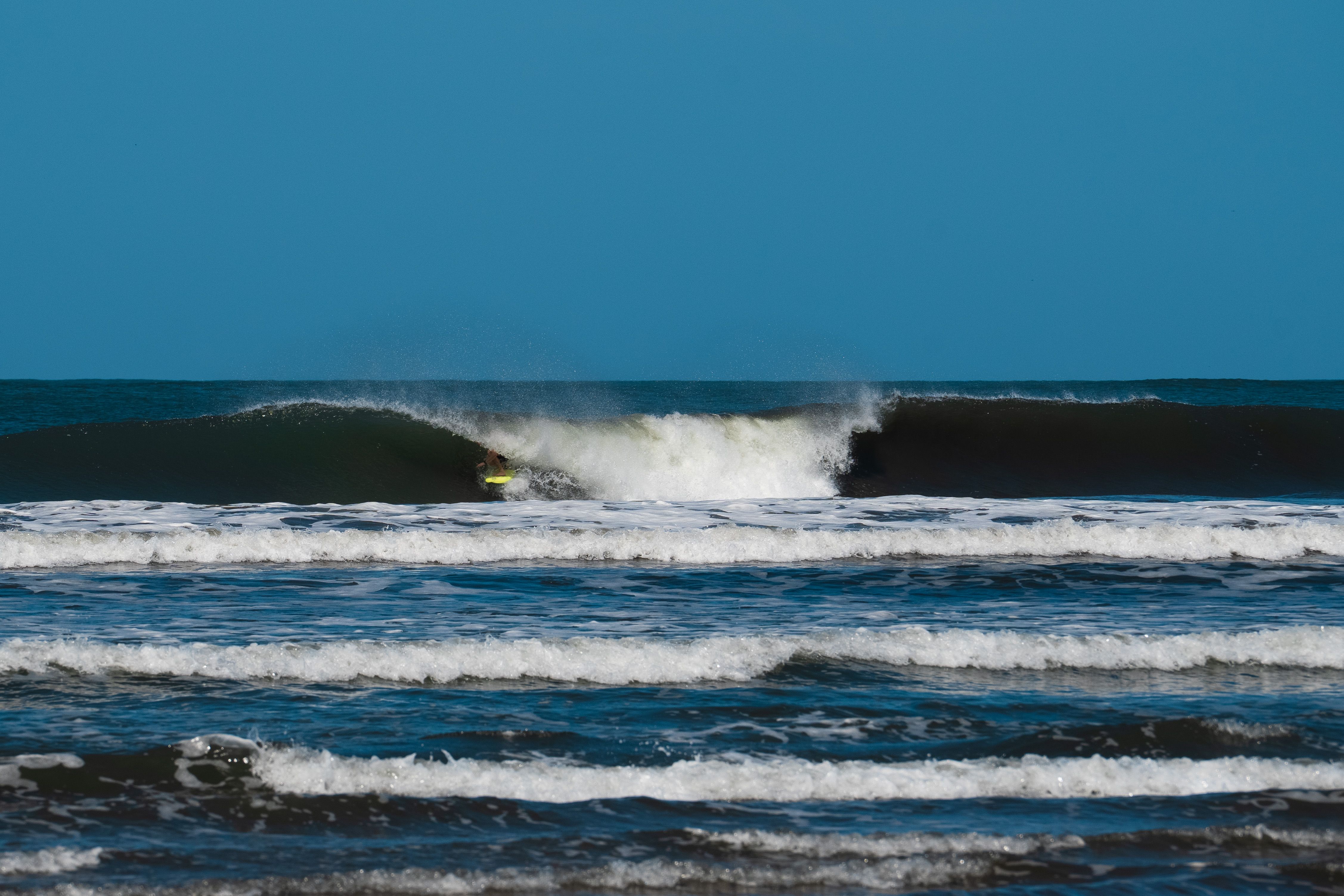
In most physics textbooks, a wave is defined as the propagation of a disturbance without net transport of matter. Yet any surfer can tell you: a good wave does carry you forward. Therefore, if surface gravity waves only transport energy, how can they entrain a whole surfboard over tens of meters?

In this article, I'll use linear Airy wave theory, weakly nonlinear corrections, and a simple dynamical model of a surfboard to explore this paradox. Along the way, we'll see how the bathymetry (the underwater topography) of a surf spot controls wave transformation and breaking, and why surfing is not possible on all kinds od waves.

Linear gravity waves and the Airy model

We consider a two-dimensional incompressible, inviscid flow under gravity, with horizontal coordinate \(x\) and vertical coordinate \(z\), where \(z=0\) corresponds to the mean free surface and \(z=-h\) to the seabed. Under the usual assumptions (small amplitude, irrotational flow), the velocity field derives from a potential \(\phi(x,z,t)\) satisfying Laplace’s equation:

\[ \nabla^2 \phi = \partial_{xx}\phi + \partial_{zz}\phi = 0, \quad -h \leq z \leq \eta(x,t), \] where \(\eta(x,t)\) denotes the free-surface elevation.

Linearizing the kinematic and dynamic boundary conditions around the flat surface \(z = 0\) leads to a sinusoidal solution for the free surface:

\[ \eta(x,t) = A \cos(kx - \omega t), \] where \(A\) is the wave amplitude, \(k\) the wavenumber, and \(\omega\) the angular frequency. The dispersion relation for surface gravity waves in finite depth is:

\[ \omega^2 = g k \tanh(kh). \]

From this we can define the phase speed \(c = \omega/k\) and identify two limiting regimes:

• Deep water (\(kh \gg 1\)): \(\tanh(kh) \approx 1\) and \(c \approx \sqrt{\frac{g}{k}}\).
• Shallow water (\(kh \ll 1\)): \(\tanh(kh) \approx kh\) and \(c \approx \sqrt{gh}\), independent of wavelength.

The associated velocity potential for a linear Airy wave reads

\[ \phi(x,z,t) = \frac{A g}{\omega} \frac{\cosh[k(z + h)]}{\cosh(kh)} \sin(kx - \omega t), \] from which we obtain the velocity components \[ u = \partial_x \phi, \quad w = \partial_z \phi. \]

g  = 9.81;
h  = 5.0;           
A  = 0.5;           
k  = 0.4;          
ω  = Sqrt[g*k*Tanh[k*h]];

η[x_, t_] := A*Cos[k*x - ω*t];

φ[x_, z_, t_] := (A*g/ω) * (Cosh[k*(z + h)]/Cosh[k*h]) * Sin[k*x - ω*t];

u[x_, z_, t_] := D[φ[x, z, t], x];
w[x_, z_, t_] := D[φ[x, z, t], z];

t0 = 0;
StreamPlot[
  {u[x, z, t0], w[x, z, t0]},
  {x, 0, 3*2*Pi/k}, {z, -h, 0},
  StreamPoints -> Fine,
  StreamStyle -> White,
  PlotRange -> All,
  FrameLabel -> (Style[#, 14, White] & /@ {"x (m)", "z (m)"}),
  Background -> Black
]

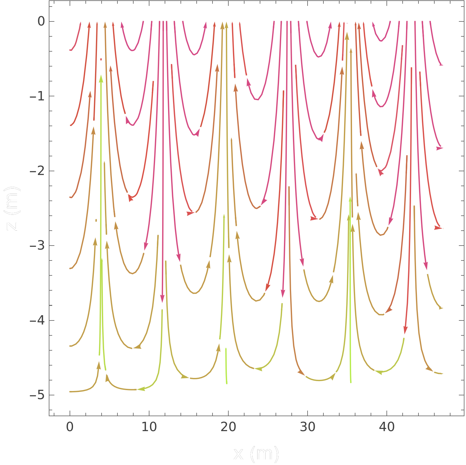
In this linear model, water particles do not follow the wave crest. Instead, they move on almost closed orbits: circular in deep water and more elliptical as the bottom is approached. Thus, purely linear waves cannot transport a fluid particle over large distances, which seems at odds with the macroscopic motion of a surfboard. The missing ingredient is hidden in the difference between linear theory and the real, finite-amplitude ocean waves that surfers encounter.

From offshore swell to breaking waves: the role of bathymetry

As waves propagate from deep to shallow water, the decreasing depth \(h(x)\) modifies the phase speed \[ c(x) = \sqrt{\frac{g}{k} \tanh(k h(x))}. \] For long waves in shallow water (\(kh \ll 1\)), this simplifies to \(c(x) \approx \sqrt{g h(x)}\), which decreases as the water becomes shallower.

Assuming negligible energy dissipation before breaking, and using the group speed \(c_g\), conservation of energy flux \(E c_g\) implies that the wave amplitude increases as the depth decreases. This process is called shoalling, and it is the reason why waves often grow taller as they approach the shore.

A simple way to illustrate this is to prescribe a gently sloping bottom profile \(h(x)\) and compute the corresponding celerity \(c(x)\) and an idealized amplitude scaling. The script below does this for a planar beach.

g = 9.81;
k = 0.4;
h0 = 20.0;       (* offshore depth *)
slope = 0.02;    (* beach slope *)

h[x_] := h0 - slope*x;

c[x_] := Sqrt[g/k*Tanh[k*h[x]]];

xmax = h0/slope - 0.1;  

Plot[
  {c[x]},
  {x, 0, xmax},
  PlotLegends -> Placed[{"c(x)"}, {0.8, 0.8}],
  AxesLabel -> (Style[#, 14, White] & /@ {"x (m)", "Phase speed (m/s)"}),
  PlotStyle -> {Directive[White, Thick]},
  Background -> Black
]

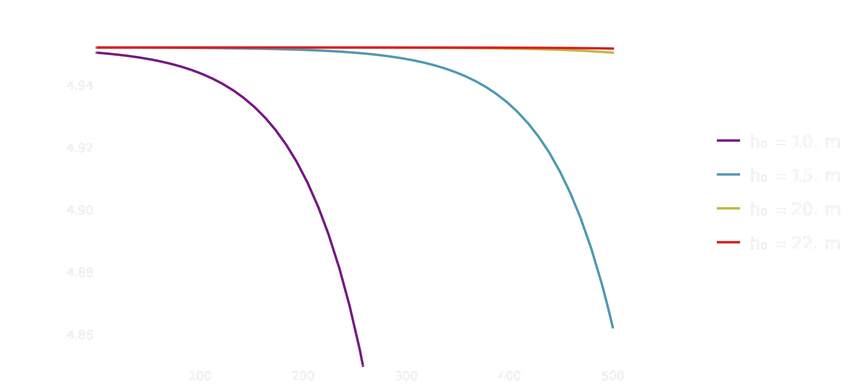
Empirically, breaking tends to occur when the wave height \(H\) reaches a fraction of the local depth: \[ H_b \approx \gamma_b\, h, \quad \gamma_b \approx 0.7 - 0.8, \] and when the slope of the free surface becomes too steep. At this point, nonlinearity is no longer small: the crest overturns, vorticity is generated, and the wave irreversibly transfers energy and momentum to the water mass.

For the surfer, this is the key transition. Before breaking, the wave mainly oscillates around an equilibrium shape. Once breaking starts, a strong, directed flow appears in the vicinity of the crest, capable of accelerating a surfboard to nearly the phase speed of the wave, provided certain conditions are met.

A minimal dynamical model of surfboard entrainment

To capture the essence of surfboard entrainment, we consider a simplified one-dimensional model. Let \(v(t)\) denote the horizontal velocity of the board and \(c\) the phase speed of the breaking wave. We assume that the board is pushed by a wave-induced force proportional to the relative velocity \(c - v\) (a crude model of hydrodynamic pressure and drag) and opposed by a viscous-type drag proportional to \(v\):

\[ m \frac{dv}{dt} = \alpha (c - v) - \beta v, \] where \(m\) is the effective mass (board + surfer), \(\alpha\) parameterizes the strength of the wave push, and \(\beta\) represents dissipative effects.

This linear ODE admits a steady state \[ v_\infty = \frac{\alpha}{\alpha + \beta} c. \] If \(\alpha \gg \beta\), then \(v_\infty \approx c\): the board is effectively captured by the wave and moves at nearly the same speed. If \(\alpha\) is too small (weak wave, poor board orientation), the board remains in a drift regime, with \(v_\infty \ll c\).

The script below integrates this equation numerically for different values of \(\alpha\), corresponding to different wave steepness or board shapes, and compares the resulting board velocity to \(c\).

m      = 80.0;    (* surfer+ board *)
cWave  = 7.0;    
β      = 20.0;    (* drag coefficient *)

alphas = {40., 80., 200.};   (* different wave push strengths *)

tmax = 6.0;

solutions =
  Table[
    NDSolve[
      {m*v'[t] == α*(cWave - v[t]) - β*v[t], v[0] == 0},
      v, {t, 0, tmax}
    ][[1]],
    {α, alphas}
  ];

Plot[
  Evaluate@Table[v[t] /. solutions[[i]], {i, Length[alphas]}] ~Join~ {cWave},
  {t, 0, tmax},
  PlotLegends -> Placed[
    Join[
      Table["v(t), α = " <> ToString[α], {α, alphas}],
      {"c (wave speed)"}
    ],
    {0.6, 0.4}
  ],
  AxesLabel -> (Style[#, 14, White] & /@ {"t (s)", "velocity (m/s)"}),
  PlotStyle -> {
    Directive[White, Thick],
    Directive[Yellow, Thick],
    Directive[Cyan, Thick],
    Directive[Red, Dashed, Thick]
  },
  Background -> Black
]

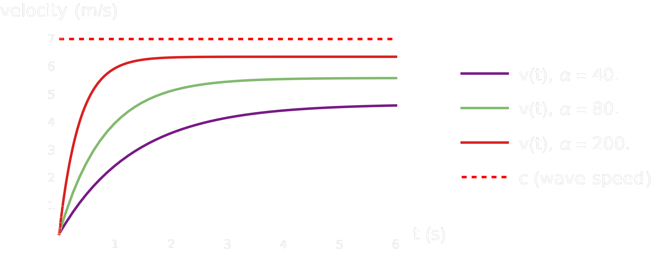
For small \(\alpha\), the board accelerates but saturates at a speed significantly lower than \(c\): the surfer experiences only a gentle push and eventually falls off the back of the wave. For large \(\alpha\), the asymptotic velocity approaches \(c\), reproducing qualitatively the sensation of “being picked up” and carried along the wave face.

References

1. 01 E. Dehandschoewercker, PhD Thesis, “Physique du Surf, ou sur l’entraînement de particules par des ondes” (2016).
2. 02 P.-Y. Lagrée, “Houle et Vagues. Ondes et Écoulements en milieu naturel”, Université Paris 6 (2023).
3. 03 A. Edwards, “The Engineering Behind Surfing”, Illumin USC (2024).