During my internship at ONERA, I explored an unusual approach to fluid simulation: using mathematical tools inspired by quantum computing to represent and manipulate large amounts of data more efficiently.
The idea is surprisingly simple. A fluid simulation may contain millions or even billions of numbers, but these numbers are not necessarily independent. If we can find an efficient way to describe the structure connecting them, perhaps we don’t need to store every single one. Better still, what if we could perform the simulation directly on that compressed representation, without ever reconstructing the original data?
That is the question I investigated using tensor networks, a family of mathematical representations closely associated with quantum computing and also used in machine learning to store data more efficiently. The results were encouraging, but they also revealed some interesting limitations.
The problem: fluid simulations get big, fast
Simulating a fluid is computationally demanding. To describe an airflow, a computer typically divides space into a large number of small cells and computes how the fluid evolves within them. The more cells we use, the finer the details we can capture, but increasing the resolution comes at a price.
Imagine a three-dimensional simulation with 1,000 points along each spatial direction. That gives
\[ 1000\times1000\times1000 = 10^9 \]
one billion grid points and depending on the numerical method, each point may store several quantities: velocities, density, or other state variables. Doubling the resolution in each direction multiplies the number of grid points by eight. This scaling makes high-resolution fluid simulation particularly expensive, in both memory and computation.
However, there is something interesting about the resulting data. A fluid field is not a collection of unrelated numbers. In many flows the velocity varies smoothly from one point to the next. Structures appear, propagate and evolve in ways that introduce correlations throughout the data. In other words, a fluid simulation often contains a considerable amount of mathematical structure, and perhaps we can exploit that structure to represent the fluid using fewer numbers. That brings us to quantum-inspired computing.
Borrowing an idea from quantum computing
Quantum computing has its own problem with enormous amounts of information. Describing a quantum system of many interacting particles can require a state space whose size grows exponentially with the number of particles. Describing the most general state of 40 quantum bits, for instance, requires \(2^{40}\), roughly one trillion complex amplitudes. This is one of the difficulties of simulating quantum systems on conventional computers.
Over the years, physicists developed mathematical tools to work around it. One important family is known as tensor networks. Rather than storing the complete state explicitly, a tensor network represents it as a collection of smaller mathematical objects connected together. When the original data has enough structure, this representation can be dramatically more compact.
An important distinction: tensor networks do not require a quantum computer. They are mathematical tools that run on ordinary computers, which makes them interesting well beyond quantum physics. One particularly convenient type is called a tensor train.
What exactly is a tensor train?
Let’s make this concrete. During my internship I developed a Mathematica package, TensorTrainTools, for constructing, manipulating and compressing tensor trains. We can use it to understand the concept without getting lost in the mathematics.
Demo 1 - turning a function into a tensor train
Consider a smooth function sampled at 1,024 equally spaced points. It might represent a wave, or a temperature profile, or realy anything else. Normally we would store it as an array of 1,024 numbers. With TensorTrainTools, we can instead reshape this array and decompose it into a tensor train:
samples = Table[
  Sin[2 Pi j/1024.] +
    0.35 Exp[-120 (j/1024. - 0.62)^2],
  {j, 0, 1023}
];

data = ArrayReshape[
  samples, ConstantArray[2, 10]
];

tt = TensorTrainDecomposition[data]
The last line of code gives this tensor train as an output:

The key operation is the decomposition: we transform a one-dimensional array into a chain of ten smaller tensors. Why ten? Because \(1024 = 2^{10}\). Every position in the original array can be labelled by ten binary digits, and the decomposition assigns one digit to each tensor. This particular approach is known as a quantized tensor train, or QTT.
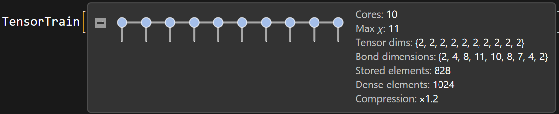
The tensor train is a chain of small blocks, called cores, each connected to its neighbours through internal links. Those connections determine how much information can be shared between different parts of the representation. The size of a connection is its bond dimension, written \(\chi\). The larger the bond dimension, the more complex the relationships the tensor train can represent, which makes \(\chi\) one of the central parameters controlling compression.
Demo 2 - how much can we compress?
A tensor train is not automatically an approximation. If we retain all the necessary information, reconstructing the original array reproduces it up to numerical precision:
reconstructed = Flatten[TensoirTrainContract[tt]];
Max[Abs[samples - reconstructed]]
Without truncation, the reconstruction error is essentially zero, apart from floating-point rounding. The real advantage appears when we deliberately discard less important components, by imposing a maximum bond dimension:
tt4 = TensorTrainDecomposition[data, "MaxBondDimension" -> 4]
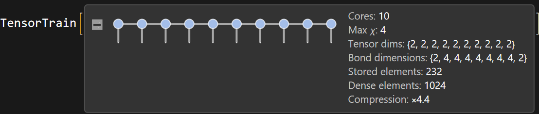
tt8 = TensorTrainDecomposition[data, "MaxBondDimension" -> 8]
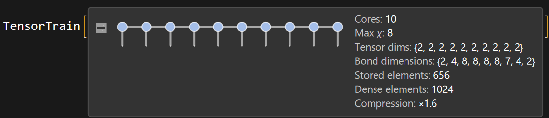
We now have two approximations of the same function: one capped at bond dimension 4, the other at 8. Reconstructing and plotting both shows how retaining more information improves the approximation.
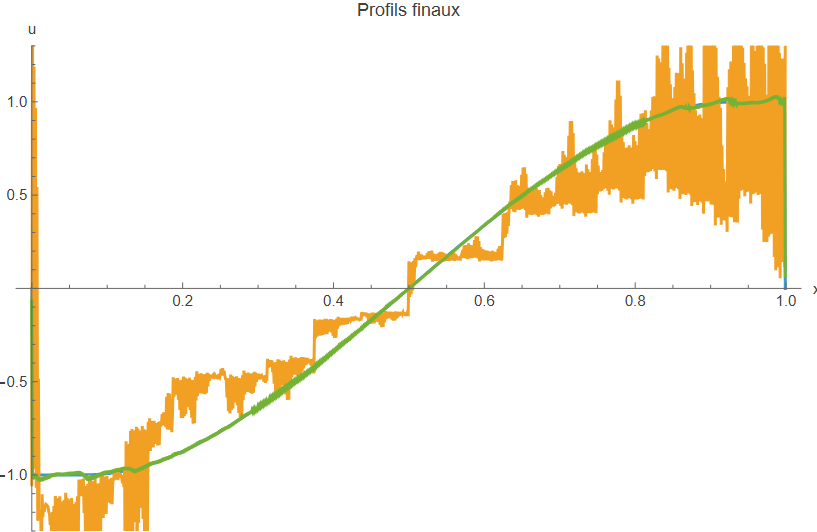
The trade-off between memory and precision is now visible. A smaller bond dimension usually means fewer parameters but greater error, a larger one allows a more accurate representation at the cost of storage. The result really depends on the structure of the data: a smooth function may need only a small bond dimension, while an irregular array can be much harder to compress.
Demo 3 - Computing directly with compressed data
One more feature of tensor trains makes them especially interesting for simulation: we can perform mathematical operations without first reconstructing the original array. TensorTrainTools supports addition, scalar multiplication and element-wise multiplication (Hadamard) directly on tensor trains. Two can be added,
sum = tt4 + tt8

or multiplied element by element,
product = TensorTrainHadamard[tt4, tt8]

and the result is itself another tensor train. These operations can increase the bond dimensions, so we generally follow them with a compression step to keep the representation manageable.
This is the key difference from ordinary file compression. When you compress a ZIP archive, you must decompress it before doing calculations. With tensor trains, we can carry out calculations while the data stays compressed. This is the property we can exploit for fluid simulation.
Finding a suitable fluid simulation method
Representing the data was only half the problem. We still needed a numerical method whose operations could be translated into tensor-network operations. During my internship, I worked on the Lattice Boltzmann method.
LBM approaches fluid mechanics differently from conventional methods that solve the Navier-Stokes equations directly. Instead of working only with macroscopic quantities such as velocity and pressure, it describes the fluid using distributions associated with a finite number of particle velocities. The algorithm has a very convenient structure: every time step consists of two operations.
Step 1 Collision: The distributions at each grid point are updated locally, through simple additions and multiplications that can also be performed on tensor trains.
Step 2 Streaming: The updated distributions move to neighbouring grid points.
The simulation repeatedly alternates between the two. The collision step was relatively straightforward to implement with tensor-train arithmetic. Streaming was more interesting: moving the values of an ordinary array is easy, but what does it mean to move a field when its individual values are no longer stored explicitly? Fortunately, there is a surprisingly elegant solution.
Shifting a fluid field using binary arithmetic
Recall that we represented the spatial index using binary digits. This means that shifting a field by one grid point is closely related to adding or subtracting 1 from a binary number. Take the number 2, written in binary as 010. Subtracting 1 gives 001.
To perform this, we start from the rightmost digit. Because it's 0, we need to borrow from its neighbour. The middle digit is 1, so it absorbs the borrow, and the leftmost digit is untouched. The surprising observation is that each digit only needs one piece of information from its neighbour: is there a borrow, or not? That is all.
By encoding that single bit of information in the connections between tensor cores, I could construct an operator that performs the entire shift directly on a tensor train. In tensor-network terminology this is a matrix product operator (MPO), and for this particular shift its bond dimension is only 2, regardless of the number of grid points.
This completed the essential ingredients. I could now perform both collision and streaming directly on compressed representations, and by assembling them into a time-stepping loop, the simulation could evolve without reconstructing the full fluid field at every step. The question was whether this compressed approach would actually produce reliable results.
Does the compressed simulation work?
For the numerical experiments, I used a simplified one-dimensional problem based on the viscous Burgers equation. It is much simpler than the full equations of three-dimensional flow, but it retains several interesting features of fluid mechanics as it is nonlinear, and has viscosity. It also has an exact solution (we can for instance use the Cole Hopf transformation to compute it) which makes it a good testing ground.
First, checking that the algorithm is correct
Before introducing any compression error, I needed to verify that the tensor-network implementation reproduced the conventional solver. I ran both versions without imposing a restrictive bond dimension, and the agreement was excellent: after a complete time step, the relative difference between the conventional solver and the tensor-train version was of order $10^{-14}$, essentially machine precision. This confirmed that the tensor-network operations reproduced the underlying algorithm. Ok, so the tensor-network formulation correctly implement the numerical method. But how much error appears when we actually compress the data? That required further investigation.
How much information does the fluid really need?
I first examined how the compressibility of the fluid field changed as resolution increased. The result was encouraging: over grids from 64 to 4,096 points, the most important components of the tensor representation remained remarkably similar. Increasing the resolution did not produce a corresponding increase in the number of components needed to capture the dominant structure of the smooth solution.
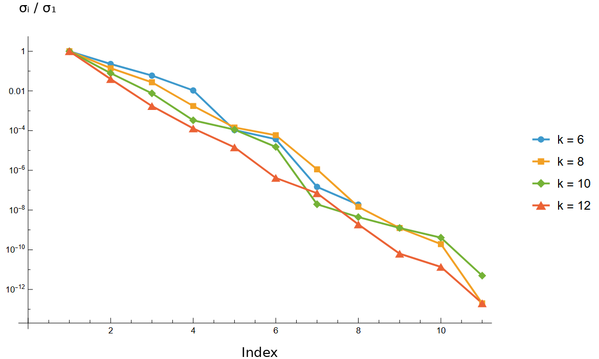
To make the observation concrete, I searched for the smallest bond dimension that kept the final compression error below a fixed threshold. For the smooth test case, a bond dimension around 6-7 (or is it 67? 😱) was sufficient across the tested resolutions. This suggests something important: doubling the number of grid points does not necessarily mean doubling the amount of information needed to describe the fluid. This concerns one test problem at a fixed accuracy target, it does not mean every flow behaves this way, but it is precisely the kind of behaviour that makes tensor-network compression promising.
What happens when we compress too much?
The next experiment varied the maximum bond dimension while keeping everything else fixed. At very small bond dimensions the error was substantial: increasing it reduced the error rapidly, almost exponentially over the tested range until further increases stopped making a meaningful difference.
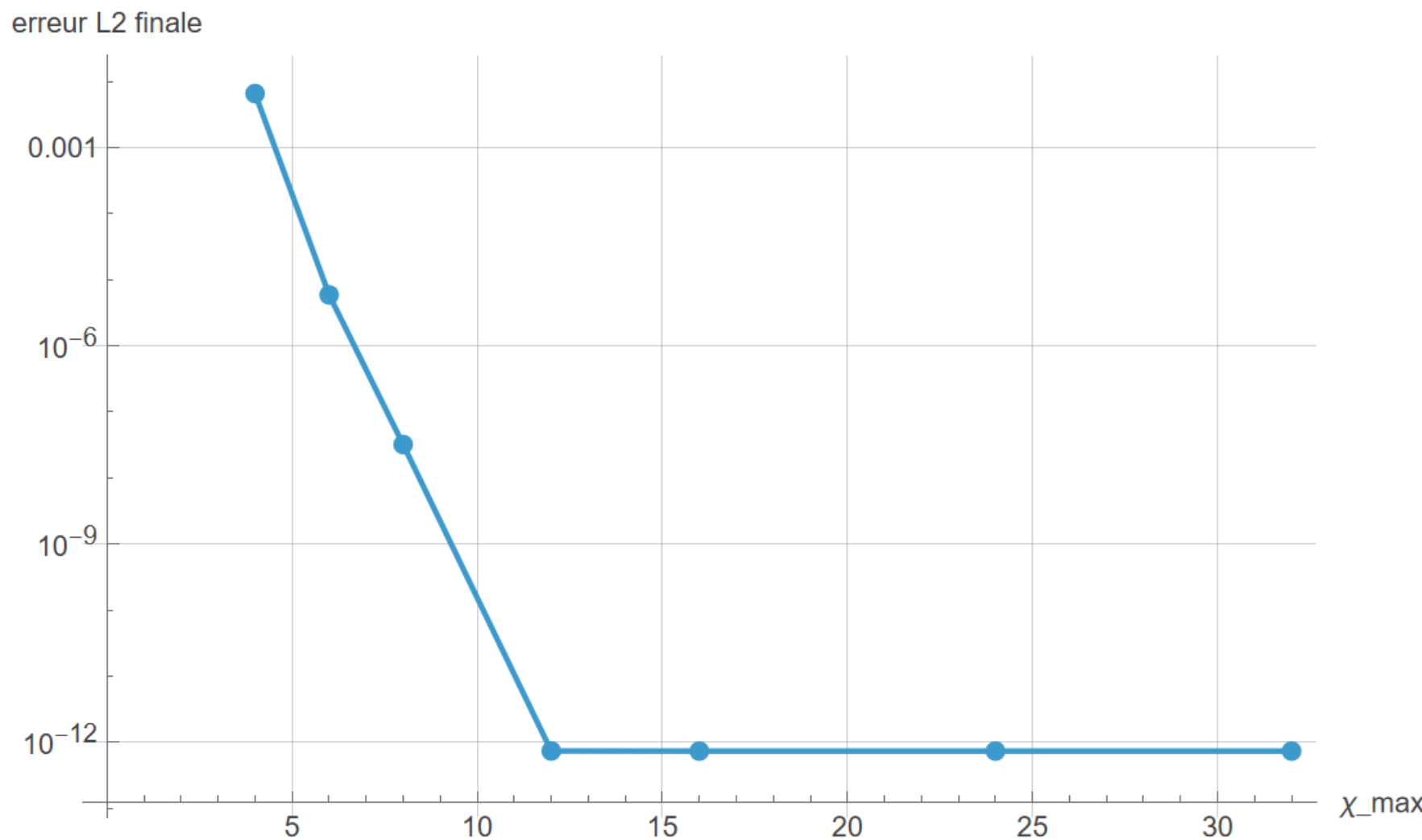
The curve reveals a familiar trade-off between compression and accuracy. At one extreme the representation is tiny but no longer accurate, at the other it retains almost everything but loses its memory advantage. Between them lies a range where a relatively small bond dimension still produces an accurate solution. The important question, then, is not simply how much can we compress? but how much can we compress while preserving the accuracy the simulation requires?
Compression introduces noise and viscosity helps control it
A more interesting phenomenon appeared when I examined how the compression error evolved over time. The compression algorithm repeatedly discards less important components of the tensor train, and each truncation introduces a small perturbation into the simulated fields. These perturbations accumulate as the simulation evolves. But a fluid has another mechanism acting in the opposite direction: viscosity, which smooths variations, dissipates small-scale disturbances and converts kinetic energy into heat.
If the disturbances stay small enough, the simulation can continue with a bounded error. But if compression is too aggressive, the perturbations may grow faster than the dynamics can control them. To test this, I repeated the simulation at different viscosities, holding the bond dimension fixed.
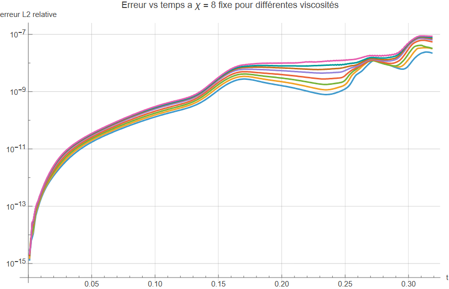
The results supported the proposed mechanism. The compression error tended to grow as viscosity decreased, and at sufficiently low bond dimensions some simulations became unstable. The interpretation is intuitive: with less dissipation to damp numerical perturbations, the algorithm becomes more sensitive to the information discarded during compression.
This is a potentially important limitation. Many interesting flows, particularly high-Reynolds-number flows, involve relatively weak viscous effects, so the approach may face its greatest difficulties precisely in the regimes where advanced fluid simulation is most useful.
Conclusions
On a simple 1D problem, I built a working compressed solver, checked it against a conventional one, and studied how compression affects accuracy and stability. Three things stood out.
More grid points don’t always mean more information. For the smooth flows I tested, the bond dimension needed for a given accuracy barely changed as resolution grew.
Compression error interacts with the physics: each truncation injects a small perturbation, and viscosity helps damp them. So the method struggles most exactly where viscosity is weak.
Smooth fields compress well, sharp features like shocks need much larger tensor ranks (similar to low viscocity flows).
The limits are clear too: real turbulent flows are far richer than 1D Burgers, so the natural next steps are 2D and 3D, and a closer look at stability at low viscosity.