
This is a deliberately small project, and that is the point. Before building a hot-wire anemomete a far more delicate instrument, I wanted to build the entire measurement chain once, end to end, on the simplest possible sensor. A Pitot probe is the easiest way to close that loop.
So the goal here is not just the probe itself but the pipeline around it: sensor → Arduino → Mathematica → live, calibrated airspeed. Everything I learn wiring, reading, filtering and calibrating this sensor carries directly over to the anemometer.
Why I’m building this
When studying fluid mechanics, it’s easy to get lost in the equations and forget the real flow behind them. I wanted to reconnect with the hands-on side by building something that lets me feel the airflow instead of only simulating it, and, more practically, to rehearse the full acquisition chain on easy hardware first.
How a Pitot tube works: a short refresher
The Pitot tube is a simple device: it measures the difference between the total pressure (where the flow stagnates) and the static pressure (of the surrounding air). That small difference corresponds directly to the kinetic energy of the moving fluid.
We start from Bernoulli’s equation for an incompressible, inviscid, steady flow along a streamline:
\[ p + \tfrac{1}{2}\rho v^2 + \rho g z = \text{const}. \]
Between a point in the free stream (velocity \(v\), pressure \(p_s\)) and the stagnation point at the tip of the tube (velocity \(0\), pressure \(p_t\)), taken at the same height, this gives
\[ p_t = p_s + \tfrac{1}{2}\rho v^2. \]
Rearranging,
\[ v = \sqrt{\dfrac{2(p_t - p_s)}{\rho}}. \]
The tube effectively measures the dynamic pressure \(\Delta p = p_t - p_s\); we then recover velocity from the relation above, adjusting for air density as needed.
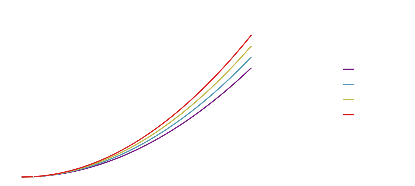
Manipulate[
  Plot[
    0.5*rho*v^2,
    {v, 0, vmax},
    Filling -> Axis
  ],
  { {rho, 1.2, "ρ (kg/m³)"}, 1.0, 1.3, 0.01 },
  { {vmax, 50, "Max velocity"}, 10, 100, 1 }
]
Time for implementation
Building the device began with the simplest possible material: PVC. Instead of metal tubing I wanted something inexpensive, easy to reproduce, and safe to drill. A short piece of small-diameter PVC pipe, the kind sold for aquarium air lines. To form the stagnation port I cut the front cleanly and smoothed it with fine sandpaper so the airflow meets a sharp, well-defined edge.
For the static ports I drilled two tiny lateral holes near the front with a 1 mm micro-bit and a hand drill. Drilling them symmetrically on opposite sides makes lateral pressure components cancel, giving a clean estimate of the true static pressure. Even this lightweight PVC probe already captures the pressure distribution Bernoulli’s law requires.
Once the ports were ready, I routed the two pressure channels through flexible PVC hoses to a differential pressure sensor. PVC is cheap, stiff enough not to collapse at low pressure, and seals well: warming the tube ends for a few seconds softens the material enough to press-fit onto the sensor barbs airtight. This makes a simple, reliable pressure line from the Pitot ports to the MPXV7002DP.
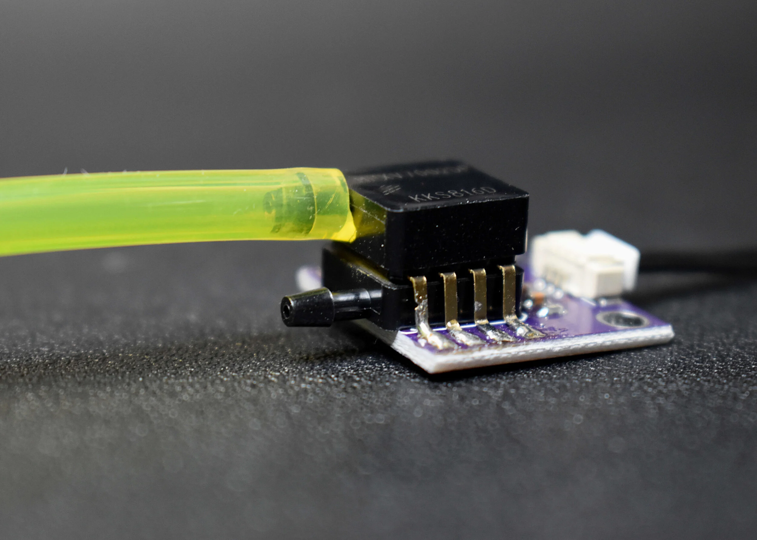
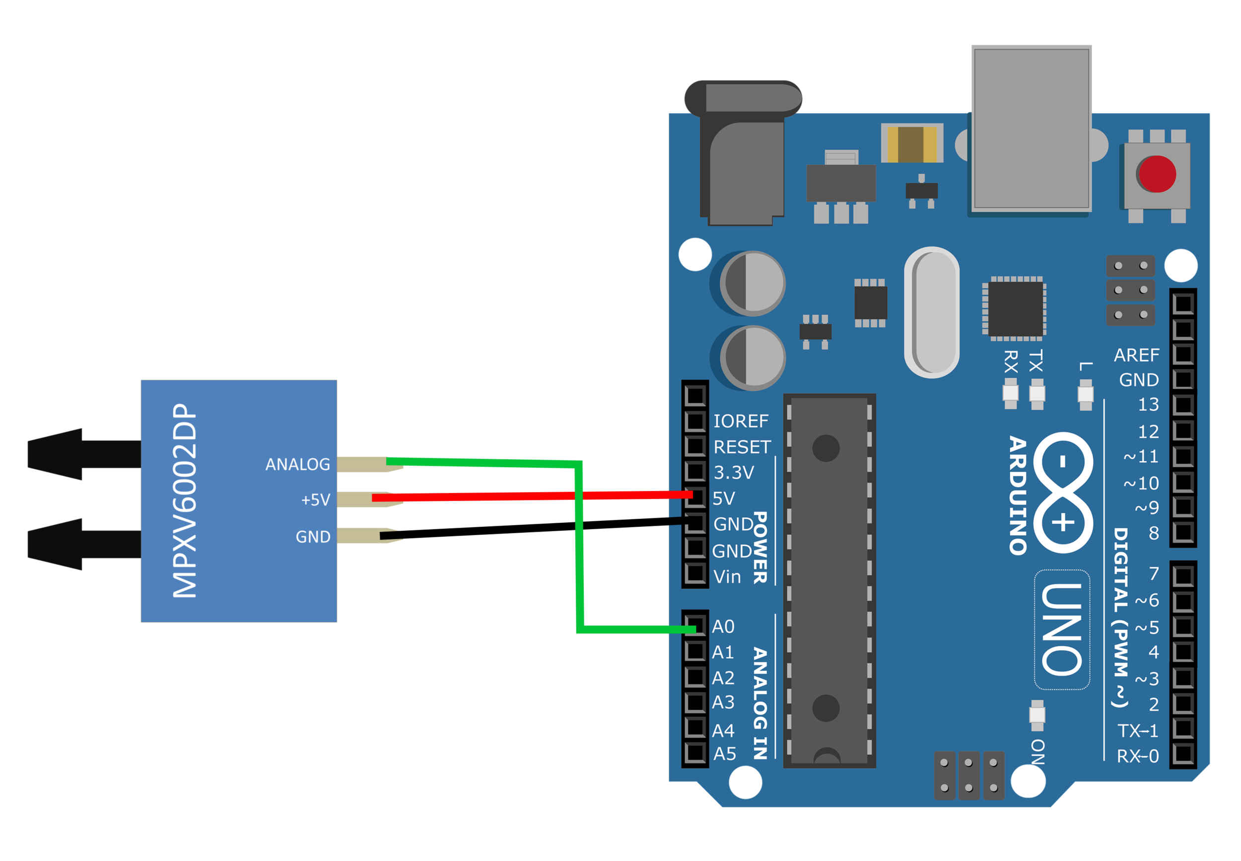
With the hardware assembled, I moved to acquisition. The MPXV7002DP outputs an analog voltage proportional to the pressure difference across its ports, so the Arduino’s ADC simply reads it on an analog input. The wiring is minimal: 5 V and GND for power, output to A0.
The Arduino sketch continuously reads the analog value, converts it to volts, subtracts the zero-pressure offset, computes \(\Delta p\) in kilopascals, and streams each measurement over USB serial. I kept the firmware deliberately short and let Mathematica handle all downstream processing and visualization.
const int pin = A0;
const float Vcc = 5.0;
const float offset = 0.5;      // Sensor output at 0 kPa
const float sensitivity = 0.5; // Volts per kPa for MPXV7002DP

void setup() {
  Serial.begin(115200);
}

void loop() {
  int raw = analogRead(pin);
  float voltage = raw * (Vcc / 1023.0);
  float dp = (voltage - offset) / sensitivity;  // Δp in kPa
  Serial.println(dp, 4);
  delay(10); // ~100 Hz
}
Connecting the Arduino to Mathematica
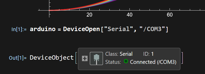
arduino = DeviceOpen["Serial", "/COM3"];

Dynamic[
  currentDP = ToExpression @ DeviceRead[arduino];
  currentDP
]
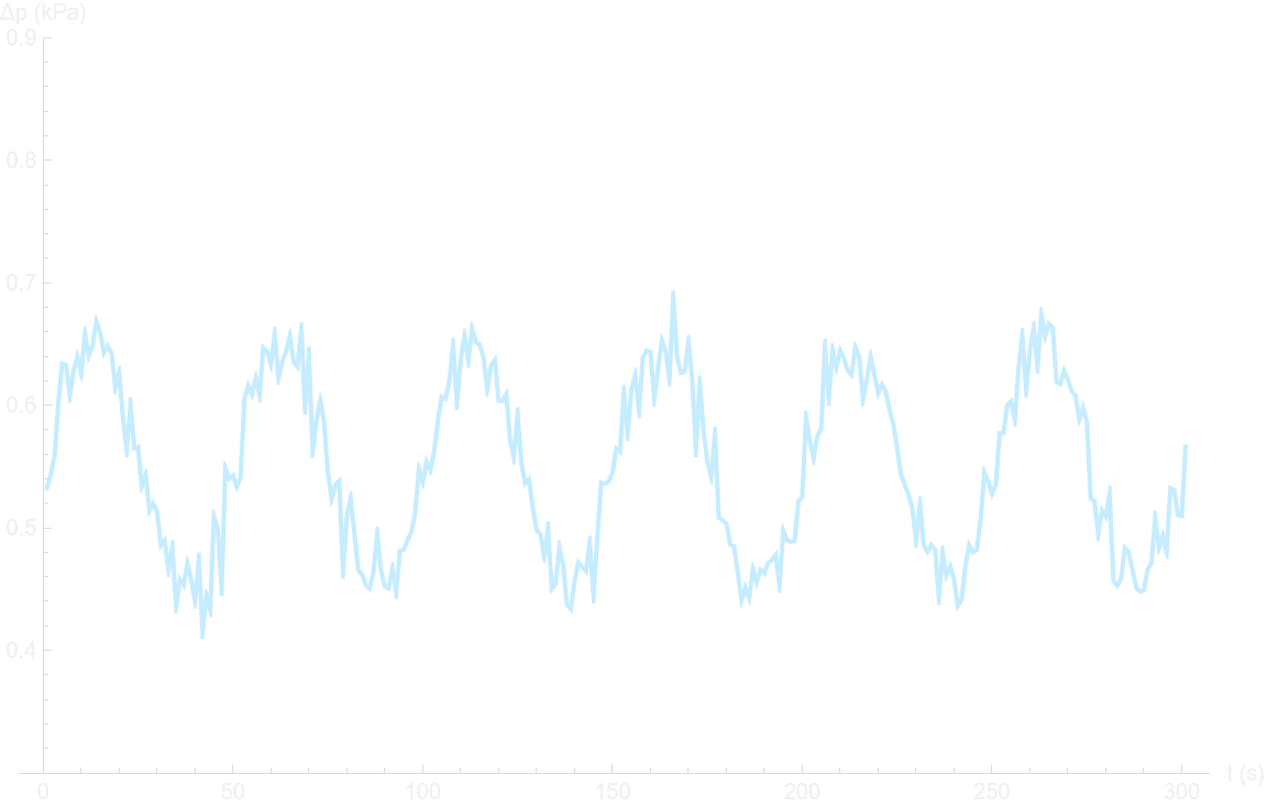
The first measurements were understandably noisy, reflecting both the sensor’s sensitivity and the turbulent airflow from a desk fan. A moving average and a simple low-pass filter, applied directly in Mathematica, immediately made the signal interpretable. Perhaps the same denoising I’ll need for the hot-wire?
Converting pressure to velocity
With a stable stream of \(\Delta p\) values, turning pressure into velocity is a direct application of Bernoulli’s relation. Taking \(\rho = 1.20~\text{kg/m}^3\),
\[ v = \sqrt{\dfrac{2\,\Delta p}{\rho}}. \]
Since the Arduino sends \(\Delta p\) in kilopascals, Mathematica converts to pascals and applies the formula. I wrapped this in a small function and used Dynamic for a live airspeed readout.
rho = 1.20; (* kg/m^3 *)

velocity[dp_] := Sqrt[2*dp*1000 / rho];  (* dp in kPa -> Pa *)

Dynamic[
  velocity[currentDP]
]
Calibration and validation
To check the system behaved realistically, I ran a simple calibration: the PVC probe at different distances in front of a fan at fixed speeds, recording \(\Delta p\) and the velocity estimate. It’s no wind tunnel, but the data followed the expected quadratic relationship between dynamic pressure and velocity.
Even with this very simple setup, the agreement was good enough to validate the concept: a low-cost PVC Pitot, a single pressure sensor, and a few lines of code turned Bernoulli’s equation into a live, interactive measurement of airspeed.